Chapter 7: ERP Analysis

This is the chapter your whole goal has been building toward. We'll first build intuition for why averaging epochs reveals a hidden signal (no EEG data needed), then apply it for real: turning Epochs into an Evoked object (the ERP), visualizing it, and comparing conditions.

Part 1: Why averaging works (a simulation)

The core problem: a single trial's brain response is usually much smaller than the ongoing noise in the signal (other brain activity, muscle tension, tiny movements). On any single trial you often can't see the response by eye at all.

But the response is time-locked to the event (same latency every time), while the noise is random (uncorrelated with the event). Average many trials together and the random noise partially cancels out, while the consistent response survives and accumulates. That average is the ERP.

import numpy as np
import matplotlib.pyplot as plt

rng = np.random.default_rng(42)

sfreq = 250
tmin, tmax = -0.2, 0.8
times = np.arange(tmin, tmax, 1 / sfreq)

# A fake "true" brain response: a bump peaking at 300 ms (like a P300).
# In reality we never get to see this directly -- it's buried in noise.
true_response = 3 * np.exp(-0.5 * ((times - 0.3) / 0.08) ** 2)

n_trials = 40
noise_amplitude = 8  # deliberately much bigger than the signal -- realistic for single-trial EEG

single_trials = np.array(
    [true_response + rng.normal(0, noise_amplitude, size=times.shape) for _ in range(n_trials)]
)

fig, axes = plt.subplots(1, 2, figsize=(12, 4), sharey=True)

axes[0].plot(times, single_trials.T, color="gray", alpha=0.3)
axes[0].plot(times, true_response, color="black", linewidth=2, label="true (hidden) response")
axes[0].set_title(f"{n_trials} single trials (each one is mostly noise)")
axes[0].legend()

axes[1].plot(times, single_trials.mean(axis=0), color="crimson", linewidth=2, label="average across trials")
axes[1].plot(times, true_response, color="black", linewidth=1, linestyle="--", label="true (hidden) response")
axes[1].set_title("Average of the trials = the ERP")
axes[1].legend()

for ax in axes:
    ax.set_xlabel("Time relative to event (s)")
    ax.axvline(0, color="k", linewidth=0.5)
axes[0].set_ylabel("Amplitude (a.u.)")
plt.tight_layout()
plt.show()

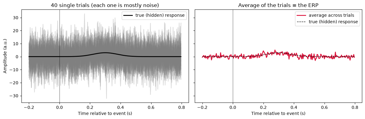
Nothing was filtered or cleaned between the two panels — the only operation was averaging. Mapped onto MNE's objects: single_trials above is what Epochs holds (one row per trial); single_trials.mean(axis=0) is exactly what epochs.average() computes, producing an Evoked object. Everything in Chapters 4–6 (filtering, ICA, rejection) exists purely to make the individual epochs less noisy so this average converges faster and cleaner — but the averaging step itself is what actually produces the ERP.

Part 2: A real ERP

Rebuilding the cleaned, epoched data from Chapters 4 and 6 (self-contained, so this notebook runs on its own):

import mne
from pathlib import Path

mne.set_log_level("WARNING")

sample_folder = Path(mne.datasets.sample.data_path()) / "MEG" / "sample"
raw = mne.io.read_raw_fif(sample_folder / "sample_audvis_raw.fif", preload=True)
events = mne.find_events(raw, stim_channel="STI 014")
event_id = {
    "auditory/left": 1,
    "auditory/right": 2,
    "visual/left": 3,
    "visual/right": 4,
}

raw.pick(["eeg", "eog"])
raw.filter(l_freq=1.0, h_freq=40.0)

epochs = mne.Epochs(
    raw,
    events,
    event_id=event_id,
    tmin=-0.2,
    tmax=0.5,
    baseline=(-0.2, 0.0),
    preload=True,
    reject=dict(eeg=150e-6, eog=250e-6),
)
epochs

	General
	MNE object type	Epochs
	Measurement date	2002-12-03 at 19:01:10 UTC
	Participant	Unknown
	Experimenter	MEG
	Acquisition
	Total number of events	269
	Events counts	auditory/left: 63 auditory/right: 69 visual/left: 72 visual/right: 65
	Time range	-0.200 – 0.499 s
	Baseline	-0.200 – 0.000 s
	Sampling frequency	600.61 Hz
	Time points	421
	Metadata	No metadata set
	Channels
	EEG	59 and 1 bad
	EOG	1
	Head & sensor digitization	146 points
	Filters
	Highpass	1.00 Hz
	Lowpass	40.00 Hz

epochs.average() → Evoked

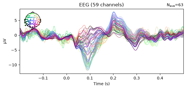
This is the one-line version of the simulation above, run on real epochs instead of fake trials.

evoked_aud_left = epochs["auditory/left"].average()
print(evoked_aud_left)
evoked_aud_left.plot(picks="eeg")
plt.show()

<Evoked | 'auditory/left' (average, N=63), -0.1998 – 0.49949 s, baseline -0.2 – 0 s, 60 ch, ~3.1 MiB>

Reading the plot: what's a "real" ERP component?

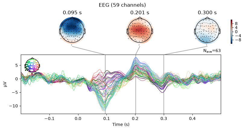
You should see a clear negative dip around 100 ms after the click — the classic N100 auditory response. plot_joint overlays the scalp topography (voltage distribution across electrodes) at the key latency, alongside the waveform — a good sanity check that a deflection is a spatially coherent brain response and not noise. A real component should look smooth and focal on the scalp map, not scattered/random.

evoked_aud_left.plot_joint(picks="eeg")
plt.show()

Quantifying a component: peak amplitude and latency

Beyond visual inspection, get_peak() finds the exact channel, time, and amplitude of the largest deflection in a time window — the kind of number you'd actually report or run statistics on.

ch_name, latency, amplitude = evoked_aud_left.get_peak(
    tmin=0.05, tmax=0.15, mode="neg", return_amplitude=True
)
print(f"Most negative deflection between 50-150 ms: {amplitude * 1e6:.2f} uV at {ch_name}, {latency * 1000:.0f} ms")

Most negative deflection between 50-150 ms: -12.00 uV at EEG 014, 90 ms

Comparing conditions

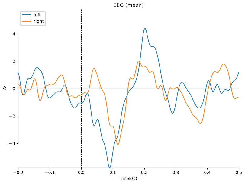
The point of most ERP studies is comparing conditions, not just looking at one. Here: left-ear vs. right-ear auditory clicks.

evoked_aud_right = epochs["auditory/right"].average()

mne.viz.plot_compare_evokeds(
    dict(left=evoked_aud_left, right=evoked_aud_right),
    picks="eeg",
    combine="mean",
)
plt.show()

A note on statistics

Eyeballing two condition curves is a starting point, not a conclusion — real ERP studies test whether a difference between conditions is statistically reliable, typically with cluster-based permutation tests (mne.stats.permutation_cluster_test and related functions), which properly handle the fact that you're testing many correlated timepoints/channels at once rather than one single comparison. That's beyond this tutorial's scope, but worth knowing the name for when you're ready to draw real conclusions from a comparison like the one above.

Summary

• epochs.average() produces an Evoked — your ERP. The single most important idea: averaging cancels random noise while a consistent, time-locked response survives.
• evoked.plot() / evoked.plot_joint() for visualizing; evoked.get_peak() for quantifying a component.
• mne.viz.plot_compare_evokeds() for comparing conditions; formal comparisons need cluster-based permutation stats.

Next: Chapter 8 — Apply This to Your Own Data