Chapter 5: Artifact Removal with ICA

Filtering (Chapter 4) removes unwanted frequencies. But eye blinks and muscle artifacts overlap in frequency with real brain signal — you can't just filter them away without also destroying real data. ICA (Independent Component Analysis) instead separates the signal spatially into statistically independent sources, so we can identify and remove specifically the artifact sources while keeping everything else.

import mne
import matplotlib.pyplot as plt
from pathlib import Path

mne.set_log_level("WARNING")

sample_folder = Path(mne.datasets.sample.data_path()) / "MEG" / "sample"
raw = mne.io.read_raw_fif(sample_folder / "sample_audvis_raw.fif", preload=True)
raw.pick(["eeg", "eog"])
raw.filter(l_freq=1.0, h_freq=40.0)  # ICA works best on data already high-pass filtered at >= 1 Hz
raw

	General
	Filename(s)	sample_audvis_raw.fif
	MNE object type	Raw
	Measurement date	2002-12-03 at 19:01:10 UTC
	Participant	Unknown
	Experimenter	MEG
	Acquisition
	Duration	00:04:38 (HH:MM:SS)
	Sampling frequency	600.61 Hz
	Time points	166,800
	Channels
	EEG	59 and 1 bad
	EOG	1
	Head & sensor digitization	146 points
	Filters
	Highpass	1.00 Hz
	Lowpass	40.00 Hz

How ICA works, conceptually

Think of your scalp electrodes as several microphones in a room with a few independent "speakers" playing simultaneously — some speakers are brain sources, one might be "eye blinks", another "muscle tension". Every electrode picks up a different mixture of all the speakers, depending on distance/geometry. ICA doesn't know which speaker is which, but it can mathematically "un-mix" the recordings back into the (assumed) independent original sources, because it looks for components that are statistically as independent from each other as possible.

Once unmixed into components, we inspect each one, decide which look like eye/muscle artifacts (based on their scalp topography and time course), and remove only those — then mix everything else back together. This is more surgical than filtering: it removes the artifact source, not a frequency band, so genuine brain signal that happens to share a frequency with the artifact survives.

ica = mne.preprocessing.ICA(n_components=15, random_state=97, max_iter="auto")
ica.fit(raw)
ica.plot_components()
plt.show()

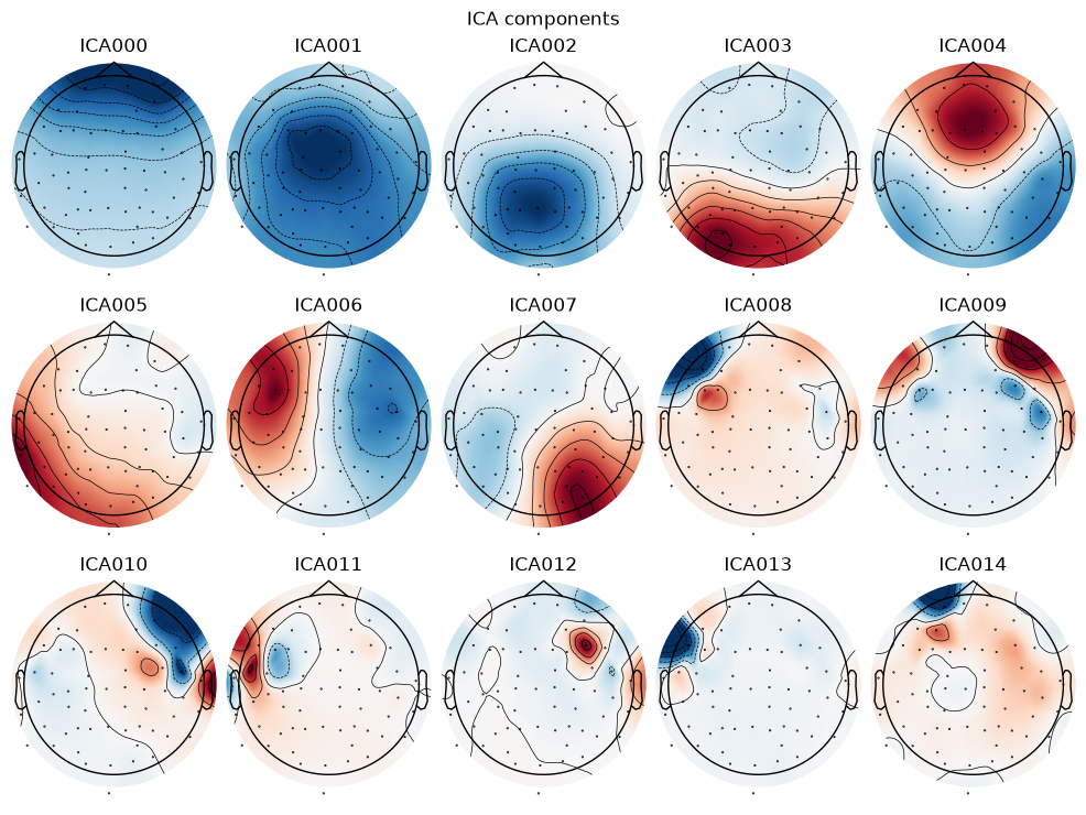
Each subplot is one component's scalp topography (which channels it contributes most strongly to). A classic eye-blink component looks like a strong, symmetric blob centered at the very front (Fp1/Fp2 area) — because blinks are the dominant frontal signal source in most recordings.

Automatic detection with an EOG channel

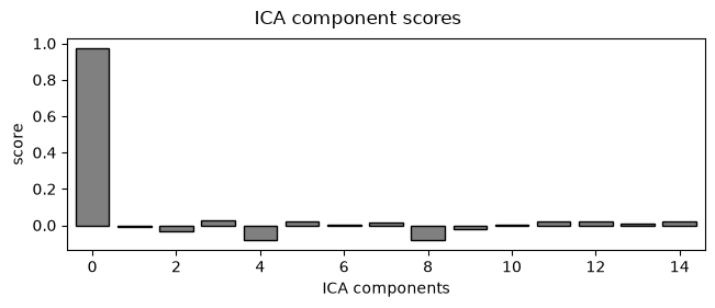
Visual inspection works, but it's subjective and slow. If your recording includes a dedicated EOG channel (this sample dataset does — it directly measures eye movement), MNE can automatically find which ICA components correlate strongly with it — far more reliable than eyeballing topographies.

eog_indices, eog_scores = ica.find_bads_eog(raw)
print("Components flagged as eye-blink related:", eog_indices)

ica.plot_scores(eog_scores)
plt.show()

Components flagged as eye-blink related: [np.int64(0)]

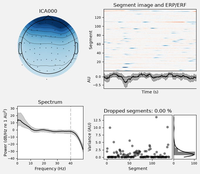
Let's look closer at the flagged component(s): its topography, time course, and how it correlates with the actual EOG signal — plot_properties bundles all of this into one diagnostic figure.

if eog_indices:
    ica.plot_properties(raw, picks=eog_indices)
    plt.show()

Excluding components and applying the cleanup

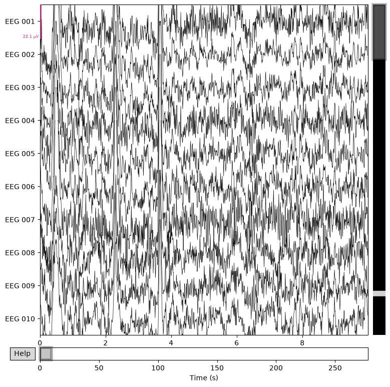
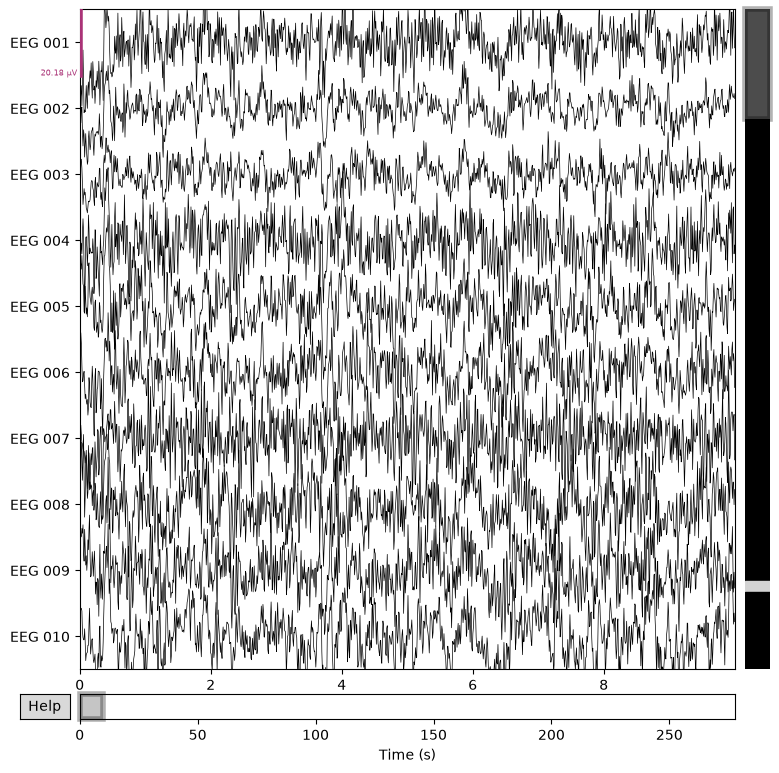
Set ica.exclude to the component indices you want removed (from either the automatic detection or your own visual inspection), then ica.apply() reconstructs the signal with those components subtracted out.

ica.exclude = eog_indices  # or set manually, e.g. [0, 3], based on what you saw above

raw_clean = raw.copy()
ica.apply(raw_clean)

raw.plot(picks="eeg", n_channels=10, duration=10, scalings="auto", title="Before ICA cleanup")
raw_clean.plot(picks="eeg", n_channels=10, duration=10, scalings="auto", title="After ICA cleanup")
plt.show()

When you don't have an EOG channel

Your own recording (32-channel, referenced to CPz) doesn't have a dedicated EOG channel — this is common. In that case:

• Fall back to visual inspection: use ica.plot_components() and ica.plot_sources(raw) (shows each component's time course, so you can literally watch for blink-shaped spikes) to identify blink/muscle-like components by eye, using the frontal-topography rule of thumb above.
• Alternatively, a simpler (blunter) fallback is amplitude-based epoch rejection after epoching — discarding whole epochs where any channel's peak-to-peak amplitude is unusually large — which we'll use as a second line of defense in Chapter 6.

Summary

• ICA separates the signal into independent components; we remove only the ones that look like eye/muscle artifacts.
• ica.find_bads_eog() automates this if an EOG channel exists; otherwise, inspect ica.plot_components() / ica.plot_sources() by eye.
• Always fit ICA on high-pass filtered (≥1 Hz) data.

Next: Chapter 6 — Events and Epoching