Chapter 1: EEG Fundamentals

New to Python entirely? Start with Chapter 0 — Getting Started first; it explains how to read any code you'll see below.

This chapter has (almost) no MNE code — it's the conceptual foundation everything else builds on. By the end you should be able to look at an EEG file's metadata and know what you're looking at.

Covered here: 1. What EEG actually measures 2. The 10-20 electrode naming system 3. Frequency bands 4. Common artifacts 5. Reference electrodes 6. Resting-state vs. task/event-based recordings

1. What is EEG actually measuring?

When large populations of neurons in the cortex fire in a synchronized, coordinated way, they generate tiny electrical fields. Electrodes on the scalp pick up the resulting voltage differences — on the order of microvolts (millionths of a volt), roughly 1,000x smaller than an ECG signal and far smaller than the noise sources around it (muscle activity, mains electricity, etc).

A few consequences of this that shape everything downstream:

• The skull and scalp smear/blur the signal spatially, so a single electrode reflects activity from a fairly large patch of cortex, not one precise "spot".
• Because the signal is so small, it's easily swamped by non-brain electrical activity (eye muscles, jaw muscles, the recording equipment itself). Most of an EEG pipeline is about isolating brain signal from this noise.
• EEG has excellent temporal resolution (millisecond-scale) but poor spatial resolution compared to something like fMRI. This is exactly why it's the tool of choice for ERPs, which are fundamentally about when something happens in the brain, not precisely where.

2. The 10-20 system

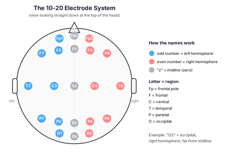
Electrode positions are standardized so results are comparable across labs and equipment. The "10-20" system places electrodes at points that are 10% or 20% of the way along measured head landmarks (nasion to inion, ear to ear). Each electrode name encodes its position:

• Letter = brain region: Fp (frontal pole), F (frontal), C (central), T (temporal), P (parietal), O (occipital)
• Number = hemisphere/distance from midline: odd = left, even = right, larger number = farther from midline
• z suffix ("zero") = midline, e.g. Cz, Pz, Oz

So C3 = central, left hemisphere; O2 = occipital, right hemisphere; Fz = frontal midline. M1/M2 (or A1/A2) are the mastoids (bone behind each ear) — commonly used as reference points rather than measuring cortex directly.

Rather than describe a diagram in words, let's generate the real thing using MNE's built-in montage — this is the exact object we used earlier to fix your own file's channel positions.

import mne
import matplotlib.pyplot as plt

mne.set_log_level("WARNING")

montage = mne.channels.make_standard_montage("standard_1020")
montage.plot(kind="topomap", show_names=True)
plt.show()

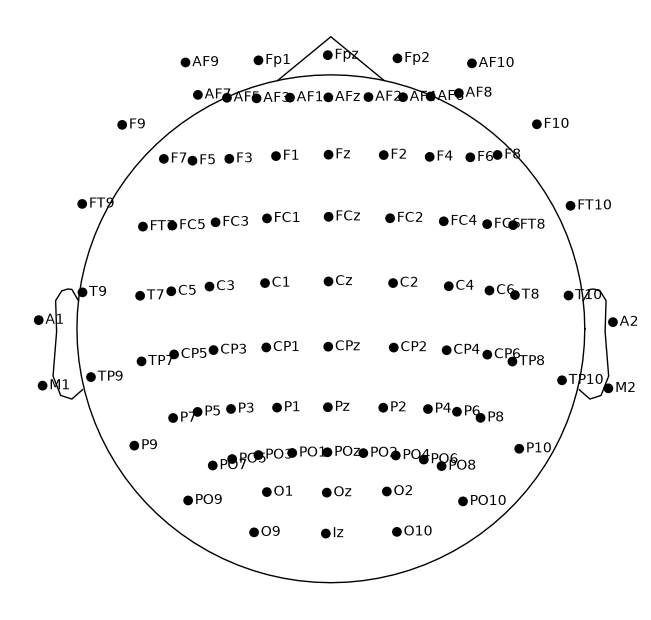
That's a top-down view of the head (nose pointing up). Find Fz, Cz, Pz, Oz running down the midline, and notice odd numbers cluster on the left, even on the right. This is the same layout your own recording's 32 channels are a subset of.

3. Frequency bands

EEG signal is often decomposed into conventional frequency bands. Rough associations (these are generalizations, not strict rules):

Band	Range	Commonly associated with
Delta (δ)	1–4 Hz	Deep sleep
Theta (θ)	4–8 Hz	Drowsiness, memory processes
Alpha (α)	8–13 Hz	Relaxed wakefulness, especially eyes closed, strongest at occipital electrodes
Beta (β)	13–30 Hz	Active thinking, focus, motor activity
Gamma (γ)	30+ Hz	High-level cognitive binding; also easily contaminated by muscle artifact

For ERP analysis specifically (your goal), you mostly don't decompose into these bands at all — you work with the raw filtered voltage waveform directly. Frequency-band analysis matters more for resting-state / oscillatory-power studies. It's still worth knowing this vocabulary because filter cutoff choices (e.g. "why 1–40 Hz?") are usually chosen with these bands in mind — a 1 Hz high-pass removes slow drift below delta, and a 40 Hz low-pass keeps everything through low gamma while cutting muscle-dominated high frequencies.

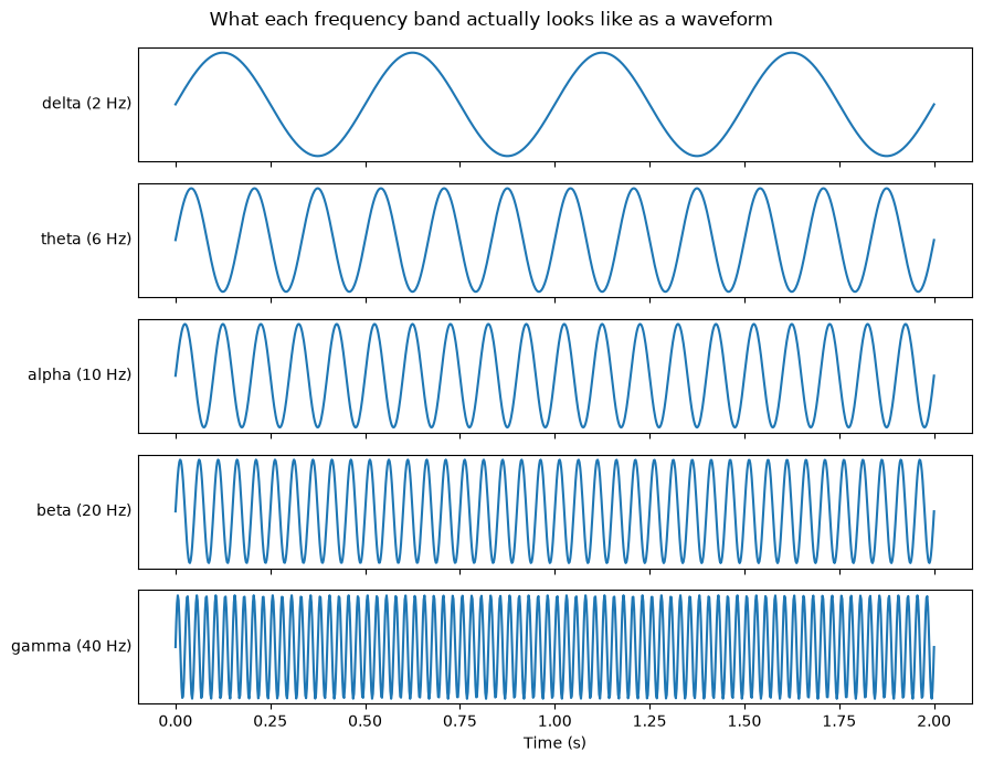
A quick visual for what these frequencies actually look like as waveforms:

import numpy as np

t = np.linspace(0, 2, 1000)
bands = {"delta (2 Hz)": 2, "theta (6 Hz)": 6, "alpha (10 Hz)": 10, "beta (20 Hz)": 20, "gamma (40 Hz)": 40}

fig, axes = plt.subplots(len(bands), 1, figsize=(9, 7), sharex=True)
for ax, (label, freq) in zip(axes, bands.items()):
    ax.plot(t, np.sin(2 * np.pi * freq * t))
    ax.set_ylabel(label, rotation=0, ha="right", va="center")
    ax.set_yticks([])
axes[-1].set_xlabel("Time (s)")
fig.suptitle("What each frequency band actually looks like as a waveform")
plt.tight_layout()
plt.show()

4. Common artifacts

Non-brain sources of electrical signal that contaminate EEG recordings:

• Eye blinks (EOG) — large, slow deflections, strongest at frontal electrodes (Fp1, Fp2). By far the most common artifact in any recording with the eyes open.
• Eye movements — smaller but similar; systematic voltage shifts as the eyeball (which is itself an electrical dipole) rotates.
• Muscle activity (EMG) — jaw clenching, frowning, swallowing. Shows up as high-frequency, spiky noise, often at temporal/frontal electrodes.
• Heartbeat (ECG) — a subtle, sharp, rhythmic pulse, more of a concern near the neck/mastoid electrodes.
• Electrical line noise — a constant sine wave at your country's mains frequency (50 Hz or 60 Hz) and its harmonics, picked up from nearby power lines/equipment. Removed with a notch filter.
• Movement / electrode artifacts — sudden jumps or drifts from a poorly-adhered electrode, cable movement, or sweat changing impedance.

Filtering handles some of this (line noise, slow drift). Eye and muscle artifacts usually need targeted removal — that's what ICA (Chapter 5) is for.

5. Reference electrodes

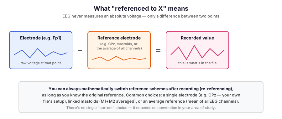
EEG measures a voltage difference — there's no such thing as an "absolute" measurement at one electrode. Every channel's value is implicitly "this electrode minus some reference point." Which reference is chosen affects the exact numbers you see, though not the underlying brain activity.

Common choices:

• A single physical electrode, e.g. Cz or CPz (this is what your own recording uses — recall the channel names like Fp1-CPz).
• Linked mastoids, averaging M1+M2 (or A1+A2) as the reference — common in ERP research since it's roughly equidistant from most scalp sites.
• Average reference, using the mean of all electrodes as the reference — common in dense-array EEG and required by some analysis methods.

You can always re-reference data after recording (MNE's set_eeg_reference(), covered in Chapter 4) as long as you know the original recording reference — you cannot recover a reference-free "true" signal, since one doesn't exist, but you can mathematically convert between reference schemes.

6. Resting-state vs. task/event-based recordings

• Resting-state: subject just sits (eyes open or closed), no stimuli. Analyzed mostly via frequency-band power (Chapter 3's table matters a lot here).
• Task/event-based (your case): the recording includes markers ("events"/"triggers"/"annotations") timestamping when something happened — a stimulus shown, a sound played, a button pressed. This lets you compute an ERP (event-related potential): cut the continuous recording into short epochs around each event, then average across many repetitions of the same event type. Averaging is the crucial step — a single trial's brain response is usually invisible in the noise, but averaging many trials cancels the random noise and reveals the consistent, time-locked response. We'll build real intuition for exactly this in Chapter 7.

Next: Chapter 2 — MNE Core Concepts, where we start writing actual MNE code and learn the vocabulary (Raw, Epochs, Evoked, Info) used throughout the rest of this tutorial.